The Evolution of Low Reynolds Number Hydrodynamics
The modeling lineage of micro-swimmers is organized around three decisions that changed what counted as a credible swimmer model. The low-Reynolds-number condition dictates that the inertial term in the momentum equation is negligible relative to viscous stress — foundational kinematic theorems demonstrate as much. This regime is defined mathematically as Re = rho U L / mu << 1. Under these specific conditions, the Navier-Stokes equations lose their non-linear convective term, becoming linear Stokes equations. Coasting is physically impossible in this environment. If propulsion stops, the swimmer halts immediately, governed entirely by the viscosity of the surrounding medium. Early modeling efforts relied heavily on kinematic reversibility to understand this flow behavior. The foundational argument for this reversibility was established in 1977 when E.M. Purcell published the scallop-theorem argument in Life at low Reynolds number.
Purely kinematic models assumed simple Newtonian fluids and onboard power. These assumptions proved physically impossible to scale down for medical applications — batteries and internal motors cannot be miniaturized to the micrometer scale while maintaining sufficient power output. The field shifted toward external magnetic actuation to overcome these micro-scale power limitations. External magnetic fields penetrate biological tissue without significant attenuation, providing a reliable energy source. A major review of magnetically actuated medical microrobots appeared in 2010, marking the transition from theoretical kinematics to applied fluid-structure interaction models. Research collaborations spanning several funding cycles during this period solidified the necessity of modeling complex, non-Newtonian biological fluids alongside external actuation. The shift required new computational frameworks capable of handling the coupled physics of magnetic torque and viscous drag.
Mechanics of Flagellated Propulsion in Viscous Media
The mechanical model is assembled by first fixing the swimmer geometry, then selecting a tail description that can exchange force and moment with the fluid. For Stokes flow, the governing fluid equations reduce to minus grad p plus mu times the Laplacian of u plus body force equal to zero, alongside div u equal to zero. Viscous forces entirely dominate inertial forces in this environment, requiring specialized mathematical treatments for the fluid-structure boundary.
A common elastic-tail representation utilizes an inextensible Euler-Bernoulli or Kirchhoff rod where the bending moment is M = EI kappa. The hydrodynamic line load is obtained by integrating surface traction around each tail cross-section. The traction vector is calculated by dotting the stress tensor with the normal vector of the surface. The fluid exerts continuous drag on the tail, which must be balanced by the elastic restoring forces of the rod structure. The mathematical coupling between the elastic deformation of the micro-robot's tail and the surrounding fluid velocity field requires precise geometric definitions to ensure numerical stability during simulation.
Geometry dictates the propulsion mechanism. A rigid helix provides a geometric mechanism for breaking time-reversal symmetry through its handedness. As the helix rotates, its handedness pushes fluid in a specific direction, generating forward thrust without violating the scallop theorem. A planar flexible tail must sustain a traveling wave rather than a reciprocal standing oscillation to accumulate forward displacement. A rigid helix can be advanced with six-degree-of-freedom kinematics, simplifying the computational load compared to fully flexible structures while maintaining accurate propulsion metrics.
Computational Strategies for Non-Newtonian Biological Fluids
Constitutive complexity is added only after the Newtonian fluid-structure implementation passes force, torque, and mesh-convergence checks. Standard Navier-Stokes solvers require significant modification to replicate blood or mucus. Shear thinning is introduced by replacing constant viscosity with the Carreau-Yasuda relation. The Carreau-Yasuda relation can be written mu(gamma_dot) = mu_infinity + (mu_0 - mu_infinity)[1 + (lambda gamma_dot)^a]^((n - 1)/a), where mu_0 and mu_infinity are limiting viscosities and lambda sets the transition timescale. This equation allows the simulated fluid to decrease in viscosity as the shear rate increases, mimicking the behavior of biological fluids under mechanical stress.
For viscoelastic formulations, the Weissenberg number Wi = lambda U/L or lambda Omega identifies when material relaxation and swimmer actuation occur on comparable timescales. High Weissenberg numbers indicate that the fluid's elasticity strongly affects the swimmer's trajectory. As the polymer chains in the fluid stretch and align with the flow, they create anisotropic viscosity and normal stress differences. Two fluids with the same apparent viscosity at one shear rate can produce different swimming speeds because their relaxation times, limiting viscosities, or elastic normal stresses differ. Capturing these differences is essential for accurate trajectory prediction in biological environments.
A practical transient convergence study can compare 50, 100, and 200 time steps per magnetic period while independently refining the near-tail mesh. Agreement from temporal refinement alone does not establish spatial convergence. Mesh deformation techniques are required to track the moving boundary of the micro-swimmer without causing numerical instability. The computational mesh must adapt dynamically as the swimmer rotates and translates through the domain.
While current fluid-structure interaction solvers provide baseline approximations, continuum FSI with a homogeneous constitutive law cannot reproduce cell-scale collisions, mucus-network rupture, wall compliance, and spatially varying tissue chemistry simultaneously; resolving those effects requires calibrated multiphase or microstructural models at substantially higher computational cost.
Simulating External Magnetic Actuation and Torque
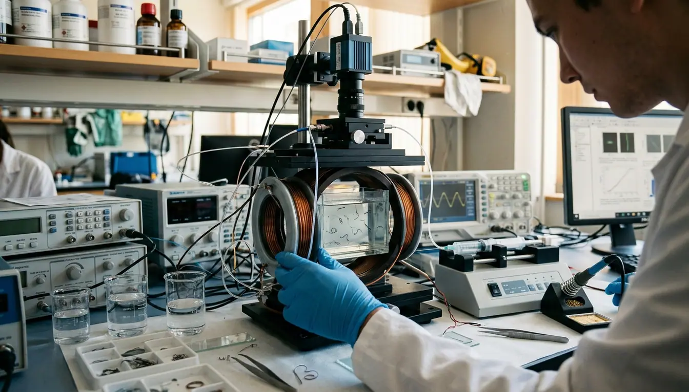
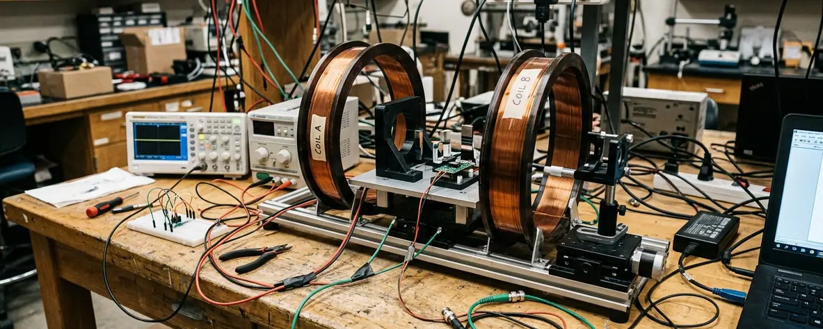
The actuation model begins with the field trajectory rather than an assumed swimmer rotation. For a permanent magnetic dipole m, the applied torque is tau_m = m cross B. In a finite head, the same total torque can be represented as a body-couple density whose volume integral equals tau_m. The solver evaluates the instantaneous magnetic torque on the head and advances the kinematic state accordingly, maintaining the coupling between the magnetic field and fluid drag at every time step.
With a rotating field defined as B(t) = B0[cos(Omega t)e1 + sin(Omega t)e2], synchronous rotation has a bounded phase lag between the head and field. Step-out begins when the required viscous torque exceeds the maximum available magnetic torque, approximately the magnitude of m cross B. As the magnetic field rotates faster, the viscous drag on the swimmer increases until synchronization is lost. Operating below the step-out frequency is critical for maintaining predictable control over the micro-robot's velocity and heading.
A simulation controller can update once per actuation period, estimate swimmer pose and phase lag, and use model-predictive or receding-horizon steering to compare candidate field axes before a bifurcation. The controller must account for the non-linear relationship between magnetic field frequency and swimmer velocity. A swimmer may remain frequency-synchronized yet show little axial progress when nearby walls redirect thrust into lateral motion or when its initial orientation approaches a hydrodynamically stable trapped state.
Case Study: Configuring a Helical Swimmer Simulation in Stokes Flow
The simulation case is configured in a sequence that isolates numerical errors. This separation keeps computational artifacts from being interpreted as fluid-structure interaction effects.
First, define the computational domain. Establish a cylindrical bounding box and apply a Carreau-Yasuda fluid model to represent shear-thinning behavior. For a baseline confinement study, set the cylinder radius to at least five swimmer-envelope radii and place the inlet and outlet at least five swimmer lengths from the initial swimmer center. Repeat this process with larger clearances to quantify boundary sensitivity and ensure the walls do not artificially inflate the calculated drag forces.
Second, initialize the geometry. Import a rigid helical tail attached to a spherical magnetic head. Resolve the narrowest head-tail junction and local helix curvature with at least three independent mesh levels. Use wall-normal inflation layers with gradual growth and report the smallest cell size relative to tail radius rather than only the total element count. Proper boundary layer resolution is required to capture the steep velocity gradients near the swimmer's surface.
Third, set boundary conditions and loads. Apply a time-dependent magnetic torque vector to the head and set the channel walls to a no-slip condition. Test nondimensional Carreau numbers Cu = lambda Omega spanning 0.1 to 10 so the runs cover near-Newtonian, transitional, and strongly rate-dependent response without assigning uncalibrated blood or mucus parameters. This parameter sweep covers fluid responses from water-like behavior to strongly shear-thinning dynamics.
Fourth, execute the solver. Run 8-12 magnetic periods as an initialization window. Verify periodicity from cycle-to-cycle displacement and phase lag, and average translational velocity over the final 3-5 complete periods. The window allows startup transients to decay before steady-state velocity is measured.
Fifth, analyze the output. Export both the shear-rate invariant and its residence time near the swimmer.
Mesh Resolution Warning: An isolated peak from a single element should trigger mesh inspection rather than be reported as a physical hotspot.
A numerically sharp shear-rate hotspot at the head-tail junction can be caused by geometric corners, poor element quality, or insufficient boundary resolution rather than by the constitutive model.
Bibliography and Authoritative Sources
The source set was chosen to connect foundational kinematics, fluid mechanics, and magnetic microrobotics rather than treating them as separate literatures. Purcell supplies the reversibility argument that underpins all subsequent low-Reynolds-number modeling.
- Purcell, E. M. (1977). Life at low Reynolds number. American Journal of Physics, 45, 3-11.
- Lauga, E., and Powers, T. R. (2009). The hydrodynamics of swimming microorganisms. Reports on Progress in Physics, 72, 096601.
- Nelson, B. J., Kaliakatsos, I. K., and Abbott, J. J. (2010). Microrobots for minimally invasive medicine. Annual Review of Biomedical Engineering, 12, 55-85.
- Lauga, E. (2020). The Fluid Dynamics of Cell Motility. Cambridge University Press.