Aerodynamic modeling becomes a controller-design issue as soon as a quadrotor leaves the low-speed envelope. A vehicle may track hover and gentle circles cleanly, then lose altitude during a fast lateral segment because its drag-free predictor allocates thrust to horizontal acceleration without reserving enough vertical authority. The useful diagnostic begins with flight-log residuals, not another round of gain tuning.
Beyond Hovering: Why Drag-Free Models Fail at High Speeds
Standard linear models treat the operating point around hover as locally representative. That approximation deteriorates during aggressive translation, where aerodynamic force grows with air-relative velocity and changes the acceleration available from a given thrust vector.
The destabilizing mechanism is usually indirect. Model mismatch drives repeated thrust or attitude saturation while the receding-horizon planner continues to assume acceleration authority that the vehicle does not possess. Each newly solved horizon inherits the same optimistic dynamics. The result can appear as altitude loss, delayed braking, or alternating constraint activity rather than an obvious aerodynamic fault.
Start With Residual Acceleration
A practical validation sweep compares predicted translational acceleration with inertial estimates after accounting for gravity, commanded thrust, and attitude. Bin the residuals by body-frame velocity component, then test whether each component follows the signed-square term v|v|. A consistent trend provides a concrete reason to extend the prediction model.
For aggressive flight, an initial NMPC configuration may use a 0.4–1.0 second prediction horizon with control updates every 10–20 milliseconds. These ranges are engineering starting points rather than universal performance guarantees. They establish the timing envelope within which added aerodynamic fidelity must earn its computational cost.
Embedding first-principles drag terms in the NMPC dynamics gives the optimizer a physically defensible estimate of available acceleration. The implementation path runs from rigid-body formulation through symbolic differentiation, embedded solver generation, and deadline-focused evaluation.
Formulating Aerodynamic Drag in the System Dynamics
The nominal rigid-body state contains 13 components: three positions, three inertial velocities, four unit-quaternion elements, and three body angular rates. A common control vector contains collective thrust and three body torques. This representation preserves the rotational dynamics required for aggressive motion while remaining compact enough for real-time optimization.
Aerodynamic force must be evaluated in the appropriate frame. Rotate inertial velocity into the body frame, apply rotor and parasitic drag there, and transform the resulting force back into the inertial equations of motion. For a lumped signed-quadratic model, each body-axis term scales with vb|vb|. A diagonal coefficient matrix is often a useful first parameterization.
Geometry can invalidate that simple symmetry. A bare X-frame may fit a symmetric diagonal drag matrix, while a camera, protective cage, or offset payload introduces cross-axis forces by changing projected area. Coefficient records should therefore identify the airframe geometry, propeller set, payload, firmware configuration, estimator revision, and flight-log interval used for fitting.
Identification and Model Boundaries
Coefficient identification needs excitation in both velocity directions on every body axis. One-sided runs can confound drag with accelerometer bias, trim error, or a constant wind component. Indoor coefficients may also shift outdoors because ground-relative velocity does not include the wind component needed to recover air-relative velocity.
A lumped model offers a workable balance between fidelity and NMPC cost. Its scope excludes deep vortex-ring-state operation, severe propeller-wing interaction, and rapidly changing wake recirculation. Trajectories entering those regimes need either a different aerodynamic state model or explicit exclusion constraints.
Quaternion handling deserves equal care. Normalize after numerical integration or control the unit norm through an algebraic or penalty treatment. Directly constraining four quaternion components while ignoring their shared norm produces an inconsistent attitude representation.
Translating Continuous Dynamics to CasADi and Acados
Implementation starts by expressing the continuous state derivative as a symbolic function of state, control, and aerodynamic parameters. The CasADi algorithmic differentiation framework supplies the Jacobians required by the nonlinear-programming and integration routines. Aerodynamic coefficients can remain online parameters, allowing updates between solves without rebuilding the generated dynamics graph.
Cost and Constraint Design
The objective usually combines state-tracking residuals with control effort. Their scaling matters more than the apparent compactness of the expression: position in metres, velocity in metres per second, angular rate in radians per second, and actuator coordinates with very different magnitudes should contribute numerically comparable weighted residuals.
Hard constraints commonly cover thrust, torque, tilt, angular rate, and obstacle geometry. Slack variables belong only on quantities whose temporary violation remains physically survivable. Actuator bounds should remain hard because the predicted trajectory has no value if it depends on unavailable thrust or torque.
Four commands per shooting node are sufficient when collective thrust and three body torques represent the actuator interface. Motor-level commands become appropriate when actuator dynamics and allocation limits must sit inside the prediction model.
Generating the Embedded Solver
The symbolic dynamics, objective, constraints, horizon, and transcription pass into Acados for optimized C-code generation. The Acados embedded optimal control documentation describes the modular solver interfaces used for this transition.
Before hardware deployment, exercise the generated solver for 10–30 seconds of closed-loop simulation under fixed seeds. Retain KKT residuals, globalization or line-search status, constraint violation, iteration count, and total solve time. A visually smooth trajectory can conceal a solver that repeatedly exits near its iteration limit.
Evaluating Solver Performance and Computational Limits
Deadline compliance and closed-loop feasibility govern solver acceptance. Average solve time alone hides the latency spikes most likely to disrupt command publication.
A defensible initial transcription uses 20–40 shooting intervals over a 0.4–1.0 second horizon. Multiple shooting exposes intermediate states and constraints, but every additional interval enlarges the optimization problem. Mesh studies should compare constraint violation and the first control action rather than relying only on overlaid trajectory plots.
SQP Configuration and Integration Accuracy
A full Sequential Quadratic Programming configuration can first establish offline whether the transcription converges reliably. Faster real-time variants may then be assessed against that reference. Nonlinear signed-quadratic drag increases derivative and integration work, so the comparison must preserve identical trajectories, constraints, and initial conditions.
One to four integration stages per shooting interval provide useful comparison points. If additional stages materially alter the first control command, the coarser discretization is not resolving the nonlinear dynamics. That result matters immediately because only the first command is applied before the horizon shifts.
Resolve the First Action: Treat a changing first control command as a discretization fault even when the predicted state curves look similar.For a 10–20 millisecond control period, measure worst-case latency across state preparation, parameter updates, integration, quadratic-program solution, and command publication. Repeated maximum-iteration exits, growing stationarity residuals, alternating active thrust constraints, and large first-interval velocity prediction errors are concrete failure signatures.
The drag model adds processing work. Its value appears when high-speed tracking produces lower short-horizon prediction residuals and fewer constraint-driven recovery maneuvers. Those paired outcomes justify the overhead more convincingly than solver timing or trajectory error viewed in isolation.
Physics-Aware Flight and Bibliography
Physics-aware autonomous flight depends on matching model complexity to the maneuver envelope. For high-velocity trajectories, calibrated aerodynamic coefficients let NMPC allocate thrust and attitude against forces the airframe will actually encounter. The same principle extends beyond quadrotors: predictive control remains credible only while its dynamics preserve the constraints that dominate execution.
Asymptotic optimality in a planning layer cannot repair a short-horizon controller that predicts unattainable acceleration. The practical boundary between planning and control therefore belongs in the evaluation record, alongside coefficient provenance, solver residuals, actuator saturation, and measured prediction error.