Bridging the Reality Gap: A Survey of Sim-to-Real Transfer Methods in Reinforcement Learning

How do we ensure a policy trained in a frictionless, perfectly observed simulation does not fail the moment it meets sensor noise and actuator latency on a physical robot? That question frames every transfer protocol that follows. The objective is concrete: convert theoretical reinforcement learning success into execution that stays inside hardware limits, recovers from contact errors, and remains task-relevant after distribution shift. Three methodological families dominate current practice—domain randomization, system identification with online adaptation, and residual reinforcement paired with imitation—and each addresses a different source of mismatch between the authority the simulator grants the learner and the information the robot actually receives.

Table of Contents

• The Sim-to-Real Dilemma: Why Do Perfect Policies Fail on Hardware?
• Characterizing the Reality Gap: Dynamics, Sensors, and Latency
• Methodology 1: Implementing Domain Randomization Protocols
• Methodology 2: System Identification and Online Adaptation
• Methodology 3: Residual Reinforcement and Imitation Learning
• Validation Protocols: Measuring Transfer Success on Physical Hardware
• The Future of Sim-to-Real: A Hybrid Approach to Policy Deployment
• Bibliography and References

The Sim-to-Real Dilemma: Why Do Perfect Policies Fail on Hardware?

The methodology begins by asking what information and authority the simulator gives the policy that the robot will not. Simulated rollouts typically expose full state, instantaneous contacts, and deterministic timing. Hardware returns delayed, partial observations and saturating actuators. Transfer design therefore divides by source of mismatch rather than by task label alone.

Domain randomization widens the training distribution until the physical plant falls inside the envelope the policy has already seen. System identification tightens the simulator until its trajectories match measured ones, then optionally trains an adaptation module that infers residual parameters online. Residual reinforcement and imitation keep an analytical or demonstrated base controller and learn only the corrective residual needed when unmodeled dynamics appear. The sections below treat these as complementary protocols, not competing slogans.

Timing bookkeeping is part of the dilemma, not an afterthought. Record the simulator step, the policy update period, the actuator command period, sensor timestamps, and command transport delay as separate quantities. Collapsing all five into one nominal control frequency conceals the phase lag that later appears as chatter or overshoot. Before any hardware deployment, replay candidate policies with observation delays swept from 0 to 40 milliseconds and with one- or two-command action holds. Policies that collapse under those replays are depending on instantaneous state feedback the robot cannot supply.

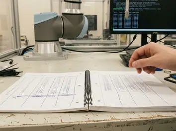
Work on asymptotically optimal motion planning at the University of Nevada, Reno, under Kostas Bekris and related NSF support including Grant CNS 0932423, has long emphasized that planning guarantees degrade when the execution model diverges from the planning model. The same discipline applies here: an RL policy inherits whatever dynamics the training loop assumed. Closing that inheritance gap is the entire transfer problem.

Characterizing the Reality Gap: Dynamics, Sensors, and Latency

Zero-shot failures concentrate on a short list of physical variables: unmodeled friction, discontinuous contact, sensor noise, encoder quantization, and control delay. A useful audit organizes around a single rollout trace. For each command, align simulated and measured joint position, velocity, motor current, contact state, and timestamp, then attribute residual error to a named mechanism rather than to a generic noise term.

Characterize static friction, Coulomb friction, viscous damping, gearbox backlash, tendon or belt compliance, encoder quantization, sensor bias, packet jitter, actuator saturation, thermal derating, and contact restitution as distinct effects. A policy may remain stable in simulation yet chatter on the robot because quantized velocity estimates pass through a derivative controller after variable communication delay. That failure mode is invisible if latency and quantization are folded into one additive disturbance.

An uncalibrated policy can repeatedly command against a hard stop, excite a flexible transmission, exceed continuous-current limits, or drive through unexpected contact. Initial runs require software joint limits, manufacturer-rated current and temperature interlocks, an independent emergency stop, a clear exclusion zone, and a tether or support fixture that does not introduce a new collision hazard.

The mathematical discrepancy is equally sharp. In simulation the problem is cast as a Markov Decision Process with transition law P(st+1|st,at) and direct access to state st. On hardware the policy receives an observation ot drawn from O(ot|st), often containing delayed measurements assembled from several physical states. Deployment is therefore a Partially Observable Markov Decision Process. Effective policies maintain a belief, a history window, or a recurrent state; memoryless maps from the latest observation to action inherit the full cost of that partial observability.

Contact remains the hardest residual. Randomizing a scalar friction coefficient does not reproduce a grasp in which fingertips alternate between sticking, slipping, rolling, and deforming the object surface. When the audit shows stick-slip or impact-dominated error, expect domain randomization alone to demand coverage that is computationally expensive and still incomplete.

Methodology 1: Implementing Domain Randomization Protocols

Prior visual transfer work established that broad appearance randomization can move deep networks from rendered scenes to camera images with little fine-tuning. Dynamics transfer extends that idea to inertial, frictional, and timing parameters, as developed in foundational research on dynamics randomization and later applied to solving complex manipulation tasks via domain randomization. The protocol below is implementation-facing.

Nominal table and parameter groups

Construct a nominal parameter table from drawings, component datasheets, and bench measurements. Group quantities by timescale. Episode-level parameters—link mass, center-of-mass offsets, camera extrinsics, background geometry—change only at reset. Step-level parameters—sensor noise draws, instantaneous latency samples, illumination flicker—resample on the communication timescale measured on the real bus.

Randomize link mass and center-of-mass offsets, joint damping, static and dynamic friction, actuator gain, command delay, contact restitution, ground compliance, camera extrinsics, focal parameters, illumination direction, light intensity, textures, and background geometry. Keep inertial parameters physically coupled: after perturbing mass distribution, recompute a positive-definite inertia tensor rather than sampling each tensor entry independently. Independent tensor entries produce nonphysical rigid bodies and teach the policy nothing transferable.

Distribution design

Use bounded uniform distributions when only engineering tolerances are known. Use truncated Gaussian distributions when repeated calibration measurements establish a central estimate and spread; truncation prevents nonphysical samples such as negative mass or an impossible focal length. A practical curriculum uses 5 to 20 second rollouts, freezes structural parameters within an episode, and resamples sensor noise or latency according to the timescale measured on the real communication path.

Domain randomization transfers visual policies well when appearance factors can be covered broadly. Discontinuous, high-dimensional contact involving stick-slip transitions, deformation, or impacts can make useful coverage computationally impractical. That limitation is structural: the method expands the training measure; it does not invent missing contact models.

Methodology 2: System Identification and Online Adaptation

Where randomization widens the prior, identification tightens the simulator against real trajectories and, when needed, trains a module that continues estimating dynamics after deployment. Calibration starts with low-excitation trajectories that isolate one mechanism at a time: gravity-dominated poses for center of mass, slow bidirectional sweeps for friction and backlash, and chirp or multisine inputs for actuator gain and latency.

Identify center-of-mass location, actuator gain, command latency, and joint friction before texture or minor compliance terms. These parameters commonly dominate gravity compensation, phase lag, and low-speed tracking while keeping the initial search dimension manageable.

Use excitation windows of 10 to 30 seconds per configuration, preceded by a stationary interval for encoder-bias and force-sensor offset estimation. Stop a run if temperature or supply voltage leaves the calibration band. Gather identification data under controlled payload, battery or bus voltage, joint-temperature range, contact surface, controller gains, and sensor-filter settings. Preserve raw timestamps and unfiltered measurements even when the deployed controller uses filtered signals; identification on filtered streams hides the very delays the adaptation module must later explain.

Online adaptation modules

After a calibrated nominal model exists, train an adaptation encoder—often a recurrent network—on history windows long enough to contain the slowest informative response. At deployment the encoder infers a latent description of the current plant without receiving the true parameter vector. Evaluate by swapping payload or friction conditions between episodes and checking whether the latent state tracks the change fast enough for the policy head to compensate.

Coupling among physical effects remains a failure mode. An adaptation network can misclassify a warm gearbox as a payload change when training varied mass and friction independently but hardware temperature changed both actuator response and joint resistance. Training curricula should therefore include joint variation of thermally linked parameters, or the latent code will assign the wrong corrective action under ordinary warm-up.

Methodology 3: Residual Reinforcement and Imitation Learning

Residual reinforcement learning deploys a base analytical controller and trains an RL policy to output only the corrective actions needed to overcome unmodeled dynamics. The base controller carries gravity compensation, nominal tracking, and safety-shaped torques; the residual fills the gap left by friction maps, compliance, and contact that the analytical model omits. Express residual actions in physical units, apply per-joint magnitude and slew-rate bounds, and train with the same saturation operator used on hardware so the policy cannot rely on corrections the actuator will discard.

Demonstration collection

Imitation supplies the residual learner—or a standalone behavioral clone—with expert trajectories collected only after observation and action interfaces match the eventual robot policy. Suitable interfaces include a six-degree-of-freedom input device for end-effector commands, bilateral master arms for joint or Cartesian teleoperation, instrumented gloves for dexterous manipulation, and kinesthetic teaching when the mechanism can be safely back-driven.

Operators perform successful trajectories plus recoveries from deliberately staged, safe disturbances. Include 20 to 60 second recovery-focused collection blocks for conditions such as a shifted object pose, a brief external push, or a partial grasp. Ordinary successful demonstrations rarely reveal the corrective behavior needed after distribution shift.

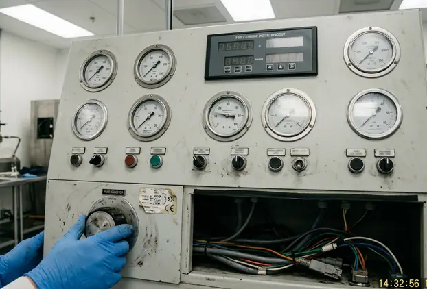
Log operator commands, robot observations, controller mode, safety interventions, camera exposure timestamps, force-torque data, and both pre-saturation and post-saturation actuator commands on a shared clock. Shared timebases are what later allow residual learning to attribute error to dynamics rather than to logging skew. The combined protocol—analytical base, residual RL, and recovery-rich imitation—bridges the reality gap by restricting the learned component to the subspace where model error actually lives.

Validation Protocols: Measuring Transfer Success on Physical Hardware

Validation advances through gates rather than leaping from simulation to unrestricted autonomy. First run the controller with motors disabled or commands shadowed. Then use supported or tethered executions. Only after log review open powered task trials under an independent human stop.

Report task success by initial-state bin together with the absolute degradation from simulation to hardware. Do not pool nominal starts, edge-of-workspace starts, and perturbation trials into one number; pooled rates hide exactly where transfer fails. Compute electrical energy from synchronized bus voltage and current when available, and report mechanical work separately when torque estimates are trustworthy. Energy comparisons require matched payload, path constraints, and completion criteria.

Measure smoothness from jerk only after documenting sampling rate and filter. Also inspect command slew, impact impulse, peak current, joint-limit margin, and intervention count. Low filtered jerk can conceal unsafe impulses that the other metrics still catch. Use 5 to 10 shadow or supported executions before powered task trials, with logs reviewed between gates.

Transfer success is not merely completion on nominal starts. A deployable policy must remain within hardware limits, detect or absorb disturbances, and return to a task-relevant state after contact errors, pushes, observation dropouts, or small payload changes.

These metrics connect directly to asymptotic optimality concerns familiar from algorithmic motion planning: a path that is optimal under an inaccurate cost or dynamics model is optimal only on paper. Hardware validation is the execution-side counterpart of that claim.

The Future of Sim-to-Real: A Hybrid Approach to Policy Deployment

Relying solely on domain randomization is insufficient for highly dynamic locomotion, impact manipulation, and dexterous contact. Randomization supplies a broad prior; it does not continuously distinguish payload change from surface friction change from actuator warm-up from observation delay once the robot is running. The deployment architecture that holds up under those conditions is hybrid.

Assign each component a distinct role. Domain randomization trains a policy prior that tolerates broad plant variation. An adaptation encoder estimates current dynamics from recent history without privileged parameter labels. A residual controller, optionally seeded by imitation, applies bounded corrections on top of an analytical or nominal base. Together they cover open-loop robustness, closed-loop plant inference, and structured correction.

Making that stack computationally feasible requires high-fidelity, differentiable simulators in which gradients pass through actuator dynamics, compliant contact, and sensor formation while respecting unilateral-contact and friction constraints. Photorealistic rendering alone does not solve dynamics transfer. Research groups should prioritize differentiable contact and actuator models with the same seriousness once reserved for visual fidelity.

Archive the simulator build, parameter priors, random seeds, controller binaries, robot calibration state, adaptation history length, and hardware log schema for every validation campaign so a physical failure can be replayed against the training assumptions. Without that archive, hybrid systems become irreproducible folklore.

Adopt the hybrid stack as the default deployment plan: randomized priors for coverage, online adaptation for plant inference, and residual control for bounded correction—backed by differentiable dynamics simulation and gated hardware validation. That combination is the methodology worth building toward; pure randomization as a standalone transfer strategy should be retired for any task where contact, impact, or rapid plant change dominate.