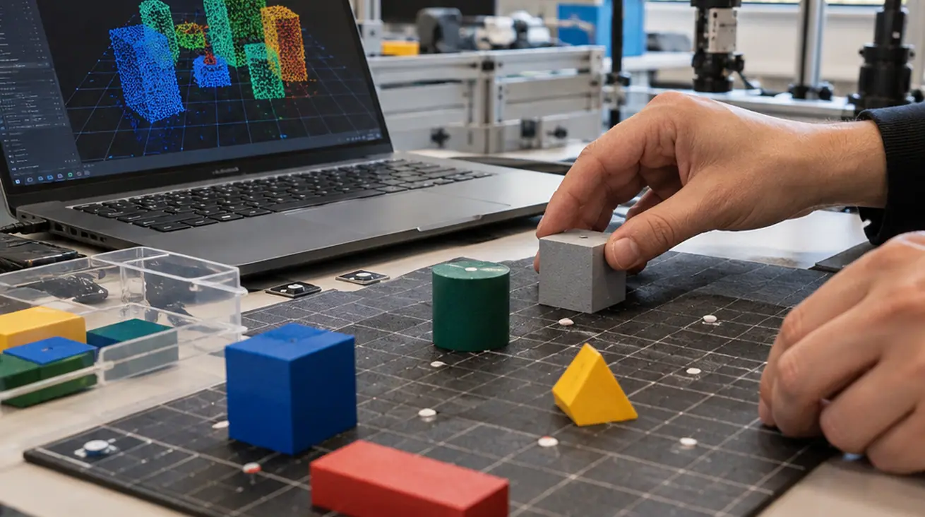
How can an autonomous system evaluate millions of possible spatial intersections in milliseconds without stalling its motion planner? The practical answer begins before any exact mesh test. Broad-phase collision detection removes object pairs that cannot intersect, leaving a smaller candidate stream for narrow-phase distance, contact, or penetration routines.
Table of Contents
- The Pair Count Before Geometry Begins
- Hash Grids and BVHs Move Memory Differently
- Turning Three-Dimensional Cells Into GPU Work
- Where Constant-Time Grid Lookup Breaks Down
- Morton-Coded Trees for Articulated Robots
- Algorithmic Sources and Lab Scope
- The 49,995,000-Pair Boundary
The Pair Count Before Geometry Begins
Earlier collision-processing accounts often concentrated on the cost of the geometric predicate: triangle overlap, convex distance, or contact generation. That leaves a more consequential question unsettled for sampling-based planning. How many configurations and object pairs reach the predicate in the first place?
Collision processing can be separated into broad phase, narrow phase, and contact or distance evaluation. For n objects, exhaustive broad-phase enumeration produces n(n−1)/2 unordered pairs before geometry rejects anything. A GPU does not make every expensive predicate cheap. Its main contribution is to prevent most pairs from reaching that predicate while processing the surviving work concurrently.
A practical device-side pipeline usually generates Axis-Aligned Bounding Boxes (AABBs), builds a spatial index, emits candidate pairs, removes duplicates, and dispatches narrow-phase kernels. These operations may run as separate kernels or as fused stages. Either design must include transforms, compaction, index construction, and synchronization in its timing.
Measure the Whole Batch
Kernel-only timing can hide the host-device seam. Uploading geometry or transforms for every query and immediately downloading a small result may cost more than the collision kernel itself.
This full-pipeline view changes the optimization target. The useful metric is complete configuration-batch latency, coupled with candidate count and narrow-phase calls, rather than raw overlap tests per second.
Hash Grids and BVHs Move Memory Differently
The relevant readings appear first in the memory layout. A compact AABB contains six scalar bounds: minimum and maximum coordinates on three axes. At 32 bits per scalar, those bounds consume 24 bytes before alignment, identifiers, child indices, or padding.
| Criterion | Spatial hash grid | Bounding Volume Hierarchy |
|---|---|---|
| Primary layout | Sorted cell keys paired with object identifiers | Leaf bounds and indexed internal nodes |
| Memory access | Adjacent threads can scan contiguous cell records | Traversal becomes less coalesced as warp lanes enter different subtrees |
| Dynamic update | Recompute occupied cells and reorder entries each step | Refit leaves and propagate child unions while topology remains useful |
| Typical advantage | Similarly sized, rapidly moving objects | Static obstacles or geometry retaining spatial locality |
These readings explain the architectural split. Hashing converts proximity into sortable records, which suits coalesced scans. BVH traversal follows child references. When threads in one 32-lane CUDA warp encounter different overlap outcomes, they descend along different paths and execute those branches with reduced parallel efficiency.
Scene evolution matters as much as traversal. A static-obstacle BVH can be built once and reused through many planning iterations. Moving links can occupy a separate refitted hierarchy or be transformed against the static tree. Hash grids instead accept reconstruction as part of each simulation step, a reasonable exchange when cell assignments already change throughout the scene.
Turning Three-Dimensional Cells Into GPU Work
Uniform grids are expected to perform well when object dimensions cluster around the selected cell width and motion invalidates spatial membership every step. The way to check that expectation is to inspect occupancy, emitted records, duplicate pairs, and complete kernel time across a representative pose sequence.
For cell width h, world position p, and grid origin o, each coordinate is computed as floor((p−o)/h). The floor operation matters for negative positions; truncation toward zero assigns cells incorrectly on opposite sides of the origin. Each thread converts an object's AABB into integer ranges on the x, y, and z axes, then emits one record for every overlapped cell.
An AABB covering ranges [ix0, ix1], [iy0, iy1], and [iz0, iz1] emits (ix1−ix0+1)(iy1−iy0+1)(iz1−iz0+1) records. A hash or linearized grid key maps each three-dimensional coordinate to a sortable one-dimensional value.
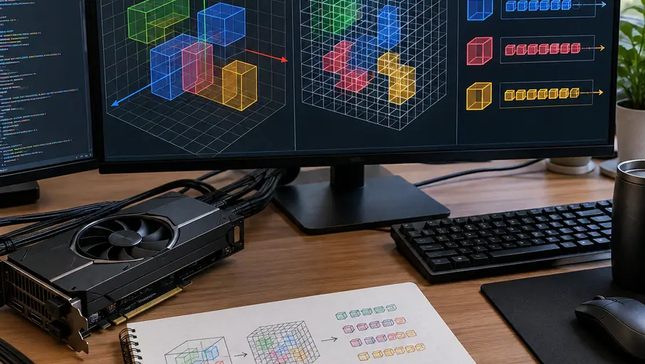
Two collisions require separate treatment. Different spatial cells may map to the same hash bucket, so the implementation must preserve complete keys or otherwise verify cell identity. A single object pair may also share several cells. Sorting packed pair identifiers removes duplicates, while canonical-cell emission prevents many duplicates from being generated.
Atomic increments fit count-and-scatter construction: threads count records per cell, a prefix sum establishes offsets, and a second pass writes object identifiers. Sorting complete key-object records offers another robust route. In swarm-like robotic scenes with comparable body sizes and bounded occupancy, the expected advantage generally holds because work remains distributed across many short cell runs.
Where Constant-Time Grid Lookup Breaks Down
A well-distributed hash function gives a uniform grid O(1) average lookup. Candidate enumeration still costs O(k) for the k records inside the queried cells. Dense occupancy can therefore erase the apparent constant-time benefit.
The sharpest geometric counterexample is the “teapot in a stadium” problem. Cells sized for the teapot force the stadium-sized object to span a huge integer range. Stadium-scale cells place many small features in the same bucket, producing long candidate lists. Neither choice preserves bounded occupancy.
BVHs respond differently to each simulation step. Updated leaf boxes propagate toward the root, with every internal AABB formed as the union of its two children. A hash grid discards and regenerates memberships as objects cross cell boundaries. This comparison should include update cost and query cost together.
✓ Pros
- Grid insertion and lookup can approach expected O(n) work when occupancy remains bounded.
- Sorted records expose contiguous memory access during cell scans.
- Rebuilding naturally tracks scenes with widespread motion.
✗ Cons
- Large AABBs may emit records across an extensive cell range.
- Dense cells create correspondingly large candidate streams.
- Repeated pair emission requires canonicalization or compaction.
Asymptotic optimality in the planner does not settle this implementation choice. A theoretically desirable planning algorithm can still spend most of its cycle waiting on poorly structured collision work.
Morton-Coded Trees for Articulated Robots
A linear BVH starts with primitive centroids. After normalization within the scene bounds, coordinate bits are interleaved into Morton keys, also called Z-order codes. A commonly described encoding uses 30-bit keys with 10 quantized bits per axis. Sorting those keys places many spatial neighbors close together; longest-common-prefix comparisons then define binary radix-tree ranges and split positions.
This construction maps well to parallel hardware. The implementation described in parallel Morton codes for BVH construction illustrates how independent threads derive internal-node relationships from sorted keys. A full binary BVH with N leaves contains N−1 internal nodes and 2N−1 total nodes, so memory planning must account for both layers.
For an articulated manipulator, leaves may represent link meshes or convex components. Internal volumes group adjacent or spatially localized parts, while self-collision masks remove known parent-child pairs before traversal emits narrow-phase work. This arrangement fits high-Degree-of-Freedom systems because rigid link geometry remains stable even as joint transforms alter world-space bounds.
Refitting proceeds from updated leaves toward the root because every parent depends on its children. Calling that operation top-down obscures the dependency. Rebuilding recomputes Morton ordering and topology; it costs more but can recover tree quality after large pose changes degrade the original grouping.
Calibrate the Rebuild
Record nodes visited, candidate pairs emitted, index-update time, and total kernel time for both refit and rebuild paths across representative robot poses. A fixed pose-count threshold has little meaning without those measurements.
Algorithmic Sources and Lab Scope
The implementation claims above follow canonical work in motion planning, spatial partitioning, collision-query software, and GPU execution semantics. For the methods discussed on this page, the University of Nevada, Reno context identifies Kostas Bekris as lead researcher and KE Bekris as co-author; NSF Grant CNS 0932423 belongs to that documented research scope rather than serving as a claim of support for this article.
Sources
- LaValle, S. M. Planning Algorithms. 2006.
- Ericson, C. Real-Time Collision Detection. 2005.
- Teschner, M., Heidelberger, B., Müller, M., Pomeranets, D., and Gross, M. “Optimized Spatial Hashing for Collision Detection of Deformable Objects.” 2003.
- Lauterbach, C., Garland, M., Sengupta, S., Luebke, D., and Manocha, D. “Fast BVH Construction on GPUs.” 2009.
- Karras, T. “Maximizing Parallelism in the Construction of BVHs, Octrees, and k-d Trees.” 2012.
- Pan, J., Chitta, S., and Manocha, D. “FCL: A General Purpose Library for Collision and Proximity Queries.” 2012. See the published account of broad-phase collision detection algorithms.
- Kavraki, L. E., Švestka, P., Latombe, J.-C., and Overmars, M. H. “Probabilistic Roadmaps for Path Planning in High-Dimensional Configuration Spaces.” 1996.
- CUDA C++ Programming Guide and OpenCL 3.0 Specification.
The 49,995,000-Pair Boundary
Broad-phase selection is a planner-latency decision. A valid benchmark reports end-to-end time alongside index updates, broad-phase candidates, narrow-phase calls, and host-device synchronization. Spatial sorting and hierarchy construction commonly target O(n log n) work. Uniform-grid insertion and lookup can approach expected O(n) work when occupancy stays bounded.
The naive alternative scales quadratically. Doubling a scene from 10,000 to 20,000 objects raises exhaustive enumeration from 49,995,000 to 199,990,000 unordered pairs, almost four times the work. At only 10,000 objects, the planner already faces 49,995,000 pair checks per frame before a single narrow-phase geometric test begins.