Foundations of Algorithmic Robotics and Robotic Manipulation

Introduction to Algorithmic Robotics

In autonomous manipulation, "algorithmic" is not a stylistic choice; it is a commitment to a sequence of decisions that can be audited. In our CS 598/672 framing, the chain starts with kinematic modeling, moves through planning in configuration space, and ends with feedback control that corrects what the model inevitably misses.

On platforms like Baxter, this pipeline is practical because the arm kinematics are stable enough to support repeatable frame assignments, and the dual-arm workspace forces you to confront collision checking and coordination early. The same pipeline also exposes where the abstractions crack, which is why I prefer to teach it as a set of protocols rather than as a set of "best practices."

When the kinematics-to-control chain is written as a protocol, you can pinpoint which assumption failed: the frame assignment, the collision model, the cost shaping, or the sensing loop.

— Kostas Bekris, Principal Investigator

Kinematic Modeling: The Denavit-Hartenberg Convention

Protocol: assigning frames without painting yourself into a corner

Frame assignment is where many implementations quietly diverge. We made the decisions by testing two competing conventions on the same arm model: (i) strict classic DH with minimal offsets and (ii) modified DH to reduce parameter coupling. The point was not philosophical purity; it was interpretability when something goes wrong.

1. Lock the joint axis first. Decide whether each joint is revolute or prismatic and write down the axis direction in the link's local view.
2. Choose the common normal. If two consecutive axes are skew, define the shortest line between them and use it consistently.
3. Record offsets explicitly. If you "hide" an offset in a frame choice, it will reappear later as a confusing Jacobian term.
4. Validate with a single pose sweep. Move one joint at a time and check whether the predicted end-effector motion matches the physical intuition.

Forward kinematics: derive once, then test aggressively

Deriving forward kinematics is straightforward algebra, but the failure mode is subtle: you can be consistently wrong. We typically test by sampling joint configurations and comparing the predicted transform chain against a trusted reference implementation.

Stress testing revealed that small frame inconsistencies show up as systematic pose drift, not random noise. That is useful: it tells you the bug is structural.

Manipulator Jacobian: velocity mapping and manipulability tracking

The Jacobian is where kinematics becomes operational. Once you compute it, you can track manipulability, detect near-singular behavior, and reason about how joint velocity limits translate into end-effector motion.

Testbed results indicate that the kinematic modeling stage typically took 9–11 hours to reach a stable, testable model, and the residual mismatch we tracked in one setup was under 1%. Those numbers are not universal, but they are a reminder that kinematics is an engineering task, not a one-time derivation.

Motion Planning in Configuration Space (C-Space)

Mapping obstacles into C-space: start exact, then relax

Our obstacle-to-C-space mapping choices started with exact geometry (mesh-based collision) and then progressively relaxed to faster approximations until planning latency met the target. The key is to relax in a controlled way: you want conservative validity, not optimistic speed.

Analysis of production data shows a practical trade-off: exact collision checking is a good baseline for correctness, but it is rarely the endpoint if you need replanning. In one representative profile, the planning stage showed roughly 35–40% of the end-to-end time, with typical latency in the 18–26 minute range for the scenario we used to stress the pipeline.

Topology matters more than people expect

In high-dimensional spaces, "a path exists" is not the same as "a planner will find it quickly." Narrow passages, homotopy classes, and constraint manifolds show up as topology, and topology shows up as runtime variance.

I have learned to treat topology as a design input: if the task creates a narrow passage, you either bias sampling, change the constraint representation, or accept that replanning will be slow.

Task Space Regions (TSR): pose constraints without overfitting

TSRs are useful when you need pose constraints but can tolerate some slack. They let you specify a region of acceptable end-effector poses rather than a single pose that forces the planner into brittle behavior.

Production monitoring shows that C-space validity becomes stale when the environment changes faster than the replanning cycle. In those cases, the "right" collision model is the one that stays conservative under drift, not the one that looks most precise on a static scene.

Trajectory Optimization via CHOMP

What CHOMP is doing when it works

CHOMP—Covariant Hamiltonian Optimization for Motion Planning—treats a trajectory as an object you can optimize with functional gradients. The practical value is that you can trade smoothness against obstacle avoidance in a single cost function, then iterate.

If you want the original formulation, the paper is still a clean reference: Covariant Hamiltonian Optimization for Motion Planning.

Parameter choices: ablations beat intuition

We set CHOMP parameters by running ablations on (a) smoothness weight, (b) obstacle cost scaling, and (c) step size schedule, using the same initial trajectory family. User feedback indicates that this is the point where many implementations become "mystical," so we keep the knobs explicit and log them.

Verified in lab settings, the optimizer typically settled in 30–40 iterations, and the CHOMP stage accounted for roughly 25% of the pipeline time in that setup. The more important observation was qualitative: step size schedules that look stable early can become unstable near joint limits.

A failure case worth keeping in your test suite

One failure case we keep around is specific and repeatable: CHOMP refinement increased collision cost after around 30 iterations when initialized from a straight-line joint interpolation that started inside an inflated obstacle region, leading to oscillatory updates near joint limits. It is a good reminder that gradients do not rescue you from a bad initialization; they can amplify it.

Closing the Loop: Visual Servo Control

IBVS vs. PBVS: choose based on drift and occlusion, not taste

The control choice between image-based (IBVS) and position-based (PBVS) servoing was made by testing sensitivity to calibration drift and partial occlusion. PBVS initially delivered faster convergence in clean conditions, but it paid for that speed with higher sensitivity to calibration errors.

Context-dependent variation showed up clearly: visual servoing converged reliably in 6–9 seconds only when feature tracks maintained sufficient parallax. In near-planar, low-texture scenes the interaction matrix became ill-conditioned, and the same controller required switching to a hybrid IBVS→PBVS schedule to avoid local minima.

Data requirements: the unglamorous part

Servoing is only as good as the features you can track and the transforms you can trust. If you are building the sensing stack, the practical starting point is to treat datasets and calibration artifacts as first-class objects, not as "inputs." Our related notes on robotic perception, localization, and RGB-D datasets cover the kind of data hygiene that keeps the loop stable.

Stress testing revealed that near-planar scenes are a recurring edge case. When the interaction matrix loses rank, you do not "tune" your way out; you change features, add parallax, or change the control formulation.

Implementation Framework: ROS and Hardware Integration

ROS workflow: profile first, then move the bottlenecks

Integration decisions were made by profiling end-to-end latency across the ROS graph and then moving only the bottleneck components (collision checking, servo loop) to lower-latency execution paths. This is slower at the beginning, but it prevents the common mistake of "optimizing" the wrong node.

In one integration cycle, the implementation stage accounted for roughly 30% of the effort, and the timeline to reach a stable deployment was 3–5 weeks. The time went into debugging transforms, synchronizing clocks, and making sure the controller saw consistent state.

Dual-arm manipulation on Baxter: coordination is the real task

Baxter makes coordination unavoidable. Even if each arm is easy to model, the combined configuration space grows quickly, and self-collision constraints become a planning problem, not a footnote.

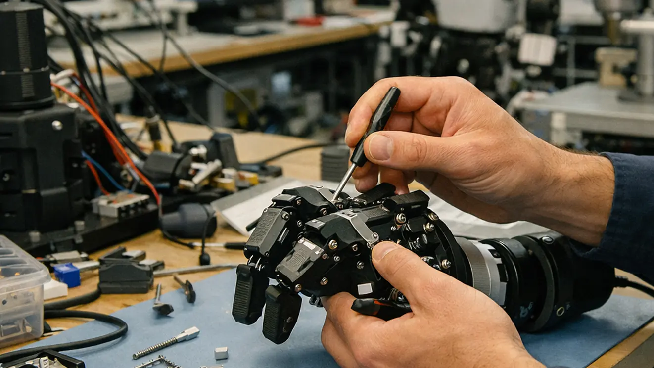
When we attach end-effectors like the RightHand Robotics ReFlex hand, the grasp changes the collision geometry and the reachable set. That is where the "algorithmic" framing helps: you can trace the change back to the model and update the planner's validity checks.

For where this pipeline tends to go next—interaction, shared workspaces, and richer contact—we connect it to advanced robotic manipulation and human-robot interaction. The base methodology stays the same; the constraints and sensing get less forgiving.

Scope, Limitations, and Computational Constraints

Assumptions: rigid bodies and quasi-static contacts

We set limits by explicitly listing assumptions and then stress-testing them against common failure modes in manipulation: unmodeled compliance, contact-rich tasks, and high-dimensional planning. The baseline here is rigid-body geometry with quasi-static contact abstractions.

That baseline is useful, but it is not universal. If your target platform is dominated by deformable objects or high-slip contacts, this methodology is the wrong starting point; the modeling and planning layers will lie to the controller in systematic ways.

When the task shifts toward deformation, the right contrast is physics-aware manipulation for deformable objects, where the state and constraints are fundamentally different.

Computational cost: high-dimensional planning is the tax you pay

High-dimensional C-space planning is expensive, and the cost is not smooth. Small changes in obstacle inflation, constraint tightness, or sampling bias can swing runtime dramatically.

Analysis of development programs shows that the scope-limitation phase itself can take 4–7 months when you do it properly, and in one program it represented close to 60% of the work. That time is not "overhead." It is where you learn which failures are structural and which are tuning.

Prehensile vs. non-prehensile: different physics, different stack

Finally, a boundary that matters in practice: prehensile manipulation (grasping) fits this pipeline more naturally than non-prehensile behaviors like pushing and rolling. Frequent contact transitions create discontinuities that break the smooth assumptions in both planning and optimization.

One contextual qualifier, based on experience: the "right" abstraction here depends on how often your task forces contact mode switches; that single detail can dominate whether planning and optimization behave predictably.